Logistic Regression with a Neural Network mindset
You will learn to:
- Build the general architecture of a learning algorithm, including:
- Initializing parameters
- Calculating the cost function and its gradient
- Using an optimization algorithm (gradient descent)
- Gather all three functions above into a main model function, in the right order.
1 - Packages
First, let’s run the cell below to import all the packages that you will need during this assignment.
- numpy is the fundamental package for scientific computing with Python.
- h5py is a common package to interact with a dataset that is stored on an H5 file.
- matplotlib is a famous library to plot graphs in Python.
- PIL and scipy are used here to test your model with your own picture at the end.
import numpy as np
import matplotlib.pyplot as plt
import h5py
import scipy
from PIL import Image
from scipy import ndimage
from lr_utils import load_dataset

%matplotlib inline
2 - Overview of the Problem set
Problem Statement: You are given a dataset (“data.h5”) containing:
- a training set of m_train images labeled as cat (y=1) or non-cat (y=0)
- a test set of m_test images labeled as cat or non-cat
- each image is of shape (num_px, num_px, 3) where 3 is for the 3 channels (RGB). Thus, each image is square (height = num_px) and (width = num_px).
You will build a simple image-recognition algorithm that can correctly classify pictures as cat or non-cat.
Let’s get more familiar with the dataset. Load the data by running the following code.
# you should make a dir called 'datasets' in your current directory在当前路径下建一个文件夹 datasets
import urllib.request
import zipfile

print("downloading with urllib...please wait...")

# download data
url_utils = 'https://raw.githubusercontent.com/andersy005/deep-learning-specialization-coursera/master/01-Neural-Networks-and-Deep-Learning/week2/Programming-Assignments/lr_utils.py'

urllib.request.urlretrieve(url_utils, 'lr_utils.py')

url_trainSet = 'https://github.com/andersy005/deep-learning-specialization-coursera/raw/master/01-Neural-Networks-and-Deep-Learning/week2/Programming-Assignments/datasets/train_catvnoncat.h5'
urllib.request.urlretrieve(url_trainSet, 'datasets/train_catvnoncat.h5')

url_testSet = 'https://github.com/andersy005/deep-learning-specialization-coursera/raw/master/01-Neural-Networks-and-Deep-Learning/week2/Programming-Assignments/datasets/test_catvnoncat.h5'
urllib.request.urlretrieve(url_testSet, 'datasets/test_catvnoncat.h5')
'''
url_data = 'https://github.com/andersy005/deep-learning-specialization-coursera/raw/master/01-Neural-Networks-and-Deep-Learning/week2/Programming-Assignments/datasets.zip'

data = urllib.request.urlopen(url_data)
with open("datasets.zip", "wb") as code:
   code.write(dataset)

# unzip datasets
with zipfile.ZipFile("datasets.zip","r") as zip_ref:
    zip_ref.extractall("")
'''
print("downloading finished!")
downloading with urllib...please wait...
downloading finished!
# Loading the data (cat/non-cat)
train_set_x_orig, train_set_y, test_set_x_orig, test_set_y, classes = load_dataset()
# Example of a picture
index = 27
plt.imshow(train_set_x_orig[index])
print ("y = " + str(train_set_y[:, index]) + ", it's a '" + classes[np.squeeze(train_set_y[:, index])].decode("utf-8") +  "' picture.")
y = [1], it's a 'cat' picture.

### START CODE HERE ### (≈ 3 lines of code)
m_train = train_set_x_orig.shape[0]
m_test = test_set_x_orig.shape[0]
num_px = train_set_x_orig.shape[1]
### END CODE HERE ###

print ("Number of training examples: m_train = " + str(m_train))
print ("Number of testing examples: m_test = " + str(m_test))
print ("Height/Width of each image: num_px = " + str(num_px))
print ("Each image is of size: (" + str(num_px) + ", " + str(num_px) + ", 3)")
print ("train_set_x shape: " + str(train_set_x_orig.shape))
print ("train_set_y shape: " + str(train_set_y.shape))
print ("test_set_x shape: " + str(test_set_x_orig.shape))
print ("test_set_y shape: " + str(test_set_y.shape))
Number of training examples: m_train = 209
Number of testing examples: m_test = 50
Height/Width of each image: num_px = 64
Each image is of size: (64, 64, 3)
train_set_x shape: (209, 64, 64, 3)
train_set_y shape: (1, 209)
test_set_x shape: (50, 64, 64, 3)
test_set_y shape: (1, 50)
# Reshape the training and test examples

### START CODE HERE ### (≈ 2 lines of code)
train_set_x_flatten = train_set_x_orig.reshape(train_set_x_orig.shape[0],-1).T
test_set_x_flatten = test_set_x_orig.reshape(test_set_x_orig.shape[0],-1).T
### END CODE HERE ###

print ("train_set_x_flatten shape: " + str(train_set_x_flatten.shape))
print ("train_set_y shape: " + str(train_set_y.shape))
print ("test_set_x_flatten shape: " + str(test_set_x_flatten.shape))
print ("test_set_y shape: " + str(test_set_y.shape))
print ("sanity check after reshaping: " + str(train_set_x_flatten[0:5,0]))
train_set_x_flatten shape: (12288, 209)
train_set_y shape: (1, 209)
test_set_x_flatten shape: (12288, 50)
test_set_y shape: (1, 50)
sanity check after reshaping: [17 31 56 22 33]
Let’s standardize our dataset.
train_set_x = train_set_x_flatten/255.
test_set_x = test_set_x_flatten/255.
Common steps for pre-processing a new dataset are:
- Figure out the dimensions and shapes of the problem (m_train, m_test, num_px, …)
- Reshape the datasets such that each example is now a vector of size (num_px * num_px * 3, 1)
- “Standardize” the data
3 - General Architecture of the learning algorithm
You will build a Logistic Regression, using a Neural Network mindset. The following Figure explains why Logistic Regression is actually a very simple Neural Network!
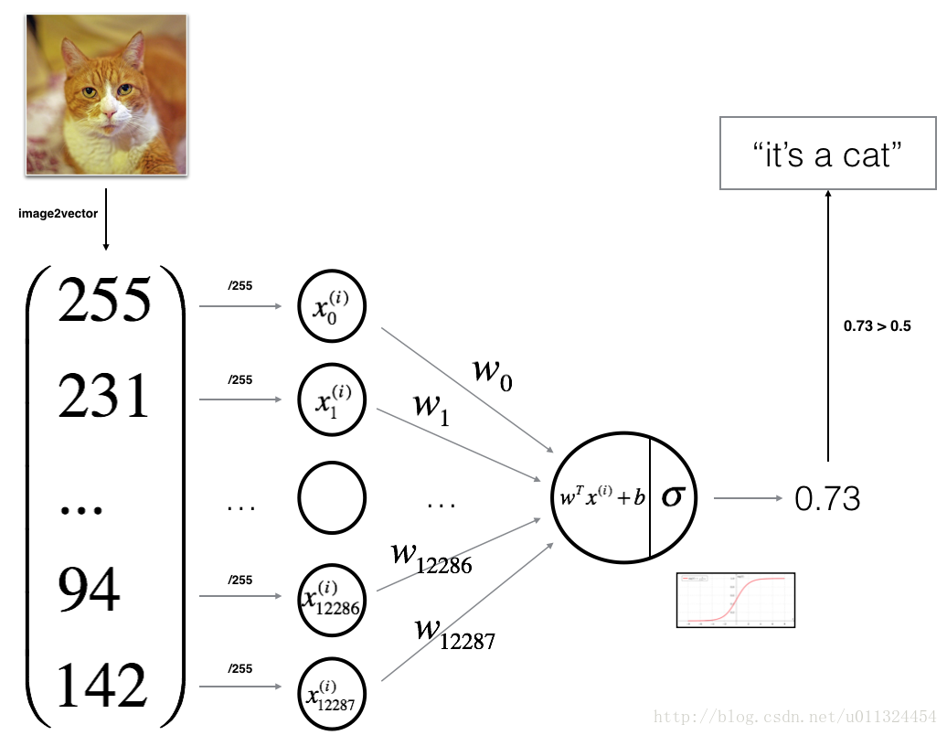
For one example \(x^{(i)}\):
\[z^{(i)} = w^T x^{(i)} + b \tag{1}\] \[\hat{y}^{(i)} = a^{(i)} = sigmoid(z^{(i)})\tag{2}\] \[\mathcal{L}(a^{(i)}, y^{(i)}) = - y^{(i)} \log(a^{(i)}) - (1-y^{(i)} ) \log(1-a^{(i)})\tag{3}\]The cost is then computed by summing over all training examples:
\[J = \frac{1}{m} \sum_{i=1}^m \mathcal{L}(a^{(i)}, y^{(i)})\tag{6}\]- Initialize the parameters of the model
- Learn the parameters for the model by minimizing the cost
- Use the learned parameters to make predictions (on the test set)
- Analyse the results and conclude
4 - Building the parts of our algorithm
- Define the model structure (such as number of input features)
- Initialize the model’s parameters
- Loop:
- Calculate current loss (forward propagation)
- Calculate current gradient (backward propagation)
- Update parameters (gradient descent)
4.1 - Helper functions
# GRADED FUNCTION: sigmoid

def sigmoid(z):
    """
    Compute the sigmoid of z

    Arguments:
    z -- A scalar or numpy array of any size.

    Return:
    s -- sigmoid(z)
    """

    ### START CODE HERE ### (≈ 1 line of code)
    s = 1 / (1 + np.exp(-z))
    ### END CODE HERE ###

    return s
print ("sigmoid([0, 2]) = " + str(sigmoid(np.array([0,2]))))
sigmoid([0, 2]) = [0.5 0.88079708]
4.2 - Initializing parameters
# GRADED FUNCTION: initialize_with_zeros

def initialize_with_zeros(dim):
    """
    This function creates a vector of zeros of shape (dim, 1) for w and initializes b to 0.

    Argument:
    dim -- size of the w vector we want (or number of parameters in this case)

    Returns:
    w -- initialized vector of shape (dim, 1)
    b -- initialized scalar (corresponds to the bias)
    """

    ### START CODE HERE ### (≈ 1 line of code)
    w = np.zeros([dim,1])
    b = 0
    ### END CODE HERE ###

    assert(w.shape == (dim, 1))
    assert(isinstance(b, float) or isinstance(b, int))

    return w, b
dim = 2
w, b = initialize_with_zeros(dim)
print ("w = " + str(w))
print ("b = " + str(b))
w = [[0.]
 [0.]]
b = 0
4.3 - Forward and Backward propagation
Forward Propagation:
- You get X
- You compute \(A = \sigma(w^T X + b) = (a^{(0)}, a^{(1)}, ..., a^{(m-1)}, a^{(m)})\)
- You calculate the cost function: \(J = -\frac{1}{m}\sum_{i=1}^{m}y^{(i)}\log(a^{(i)})+(1-y^{(i)})\log(1-a^{(i)})\)
Here are the two formulas you will be using:
# GRADED FUNCTION: propagate

def propagate(w, b, X, Y):
    """
    Implement the cost function and its gradient for the propagation explained above

    Arguments:
    w -- weights, a numpy array of size (num_px * num_px * 3, 1)
    b -- bias, a scalar
    X -- data of size (num_px * num_px * 3, number of examples)
    Y -- true "label" vector (containing 0 if non-cat, 1 if cat) of size (1, number of examples)

    Return:
    cost -- negative log-likelihood cost for logistic regression
    dw -- gradient of the loss with respect to w, thus same shape as w
    db -- gradient of the loss with respect to b, thus same shape as b

    Tips:
    - Write your code step by step for the propagation. np.log(), np.dot()
    """

    m = X.shape[1]

    # FORWARD PROPAGATION (FROM X TO COST)
    ### START CODE HERE ### (≈ 2 lines of code)
    A = sigmoid(np.dot(w.T,X) + b)                                     # compute activation
    cost = -1/m * (np.dot(Y,np.log(A).T) + np.dot((1-Y),np.log(1 - A).T))                                  # compute cost
    ### END CODE HERE ###

    # BACKWARD PROPAGATION (TO FIND GRAD)
    ### START CODE HERE ### (≈ 2 lines of code)
    dw = 1 / m *(np.dot(X,(A - Y).T))
    db = 1 / m *(np.sum(A - Y))
    ### END CODE HERE ###

    assert(dw.shape == w.shape)
    assert(db.dtype == float)
    cost = np.squeeze(cost)
    assert(cost.shape == ())

    grads = {"dw": dw,
             "db": db}

    return grads, cost
w, b, X, Y = np.array([[1],[2]]), 2, np.array([[1,2],[3,4]]), np.array([[1,0]])
grads, cost = propagate(w, b, X, Y)
print ("dw = " + str(grads["dw"]))
print ("db = " + str(grads["db"]))
print ("cost = " + str(cost))
dw = [[0.99993216]
 [1.99980262]]
db = 0.49993523062470574
cost = 6.000064773192205
Optimization
- You have initialized your parameters.
- You are also able to compute a cost function and its gradient.
- Now, you want to update the parameters using gradient descent.
Exercise: Write down the optimization function. The goal is to learn $w$ and $b$ by minimizing the cost function $J$. For a parameter $\theta$, the update rule is $ \theta = \theta - \alpha \text{ } d\theta$, where $\alpha$ is the learning rate.
# GRADED FUNCTION: optimize

def optimize(w, b, X, Y, num_iterations, learning_rate, print_cost = False):
    """
    This function optimizes w and b by running a gradient descent algorithm

    Arguments:
    w -- weights, a numpy array of size (num_px * num_px * 3, 1)
    b -- bias, a scalar
    X -- data of shape (num_px * num_px * 3, number of examples)
    Y -- true "label" vector (containing 0 if non-cat, 1 if cat), of shape (1, number of examples)
    num_iterations -- number of iterations of the optimization loop
    learning_rate -- learning rate of the gradient descent update rule
    print_cost -- True to print the loss every 100 steps

    Returns:
    params -- dictionary containing the weights w and bias b
    grads -- dictionary containing the gradients of the weights and bias with respect to the cost function
    costs -- list of all the costs computed during the optimization, this will be used to plot the learning curve.

    Tips:
    You basically need to write down two steps and iterate through them:
        1) Calculate the cost and the gradient for the current parameters. Use propagate().
        2) Update the parameters using gradient descent rule for w and b.
    """

    costs = []

    for i in range(num_iterations):


        # Cost and gradient calculation (≈ 1-4 lines of code)
        ### START CODE HERE ###
        grads, cost = propagate(w,b,X,Y)
        ### END CODE HERE ###

        # Retrieve derivatives from grads
        dw = grads["dw"]
        db = grads["db"]

        # update rule (≈ 2 lines of code)
        ### START CODE HERE ###
        w = w - learning_rate*dw
        b = b - learning_rate*db
        ### END CODE HERE ###

        # Record the costs
        if i % 100 == 0:
            costs.append(cost)

        # Print the cost every 100 training examples
        if print_cost and i % 100 == 0:
            print ("Cost after iteration %i: %f" %(i, cost))

    params = {"w": w,
              "b": b}

    grads = {"dw": dw,
             "db": db}

    return params, grads, costs
params, grads, costs = optimize(w, b, X, Y, num_iterations= 100, learning_rate = 0.009, print_cost = False)

print ("w = " + str(params["w"]))
print ("b = " + str(params["b"]))
print ("dw = " + str(grads["dw"]))
print ("db = " + str(grads["db"]))
w = [[0.1124579 ]
 [0.23106775]]
b = 1.5593049248448891
dw = [[0.90158428]
 [1.76250842]]
db = 0.4304620716786828
Exercise: The previous function will output the learned w and b. We are able to use w and b to predict the labels for a dataset X. Implement the predict() function. There is two steps to computing predictions:
Calculate \(\hat{Y} = A = \sigma(w^T X + b)\)
Convert the entries of a into 0 (if activation <= 0.5) or 1 (if activation > 0.5), stores the predictions in a vector Y_prediction. If you wish, you can use an if/else statement in a for loop (though there is also a way to vectorize this).
# GRADED FUNCTION: predict

def predict(w, b, X):
    '''
    Predict whether the label is 0 or 1 using learned logistic regression parameters (w, b)

    Arguments:
    w -- weights, a numpy array of size (num_px * num_px * 3, 1)
    b -- bias, a scalar
    X -- data of size (num_px * num_px * 3, number of examples)

    Returns:
    Y_prediction -- a numpy array (vector) containing all predictions (0/1) for the examples in X
    '''

    m = X.shape[1]
    Y_prediction = np.zeros((1,m))
    w = w.reshape(X.shape[0], 1)

    # Compute vector "A" predicting the probabilities of a cat being present in the picture
    ### START CODE HERE ### (≈ 1 line of code)
    A = sigmoid(np.dot(w.T,X) + b)
    ### END CODE HERE ###

    for i in range(A.shape[1]):

        # Convert probabilities A[0,i] to actual predictions p[0,i]
        ### START CODE HERE ### (≈ 4 lines of code)
        if(A[0][i] <= 0.5):
            Y_prediction[0][i] = 0
        else:
            Y_prediction[0][i] = 1
        ### END CODE HERE ###

    assert(Y_prediction.shape == (1, m))

    return Y_prediction
print ("predictions = " + str(predict(w, b, X)))
predictions = [[1. 1.]]
5 - Merge all functions into a model
ou will now see how the overall model is structured by putting together all the building blocks (functions implemented in the previous parts) together, in the right order.
Exercise: Implement the model function. Use the following notation:
- Y_prediction for your predictions on the test set
- Y_prediction_train for your predictions on the train set
- w, costs, grads for the outputs of optimize()
# GRADED FUNCTION: model

def model(X_train, Y_train, X_test, Y_test, num_iterations = 2000, learning_rate = 0.5, print_cost = False):
    """
    Builds the logistic regression model by calling the function you've implemented previously

    Arguments:
    X_train -- training set represented by a numpy array of shape (num_px * num_px * 3, m_train)
    Y_train -- training labels represented by a numpy array (vector) of shape (1, m_train)
    X_test -- test set represented by a numpy array of shape (num_px * num_px * 3, m_test)
    Y_test -- test labels represented by a numpy array (vector) of shape (1, m_test)
    num_iterations -- hyperparameter representing the number of iterations to optimize the parameters
    learning_rate -- hyperparameter representing the learning rate used in the update rule of optimize()
    print_cost -- Set to true to print the cost every 100 iterations

    Returns:
    d -- dictionary containing information about the model.
    """

    ### START CODE HERE ###

    # initialize parameters with zeros (≈ 1 line of code)
    w, b = initialize_with_zeros(X_train.shape[0])

    # Gradient descent (≈ 1 line of code)
    parameters, grads, costs =  optimize(w, b, X_train, Y_train, num_iterations, learning_rate, print_cost)

    # Retrieve parameters w and b from dictionary "parameters"
    w = parameters["w"]
    b = parameters["b"]

    # Predict test/train set examples (≈ 2 lines of code)
    Y_prediction_test = predict(w, b, X_test)
    Y_prediction_train = predict(w, b, X_train)

    ### END CODE HERE ###

    # Print train/test Errors
    print("train accuracy: {} %".format(100 - np.mean(np.abs(Y_prediction_train - Y_train)) * 100))
    print("test accuracy: {} %".format(100 - np.mean(np.abs(Y_prediction_test - Y_test)) * 100))


    d = {"costs": costs,
         "Y_prediction_test": Y_prediction_test,
         "Y_prediction_train" : Y_prediction_train,
         "w" : w,
         "b" : b,
         "learning_rate" : learning_rate,
         "num_iterations": num_iterations}

    return d
Run the following cell to train your model.
d = model(train_set_x, train_set_y, test_set_x, test_set_y, num_iterations = 2000, learning_rate = 0.005, print_cost = True)
Cost after iteration 0: 0.693147
Cost after iteration 100: 0.584508
Cost after iteration 200: 0.466949
Cost after iteration 300: 0.376007
Cost after iteration 400: 0.331463
Cost after iteration 500: 0.303273
Cost after iteration 600: 0.279880
Cost after iteration 700: 0.260042
Cost after iteration 800: 0.242941
Cost after iteration 900: 0.228004
Cost after iteration 1000: 0.214820
Cost after iteration 1100: 0.203078
Cost after iteration 1200: 0.192544
Cost after iteration 1300: 0.183033
Cost after iteration 1400: 0.174399
Cost after iteration 1500: 0.166521
Cost after iteration 1600: 0.159305
Cost after iteration 1700: 0.152667
Cost after iteration 1800: 0.146542
Cost after iteration 1900: 0.140872
train accuracy: 99.04306220095694 %
test accuracy: 70.0 %
Expected Output:
Train Accuracy 99.04306220095694 % Test Accuracy 70.0 % Comment: Training accuracy is close to 100%. This is a good sanity check: your model is working and has high enough capacity to fit the training data. Test error is 68%. It is actually not bad for this simple model, given the small dataset we used and that logistic regression is a linear classifier. But no worries, you’ll build an even better classifier next week!
Also, you see that the model is clearly overfitting the training data. Later in this specialization you will learn how to reduce overfitting, for example by using regularization. Using the code below (and changing the index variable) you can look at predictions on pictures of the test set.
# Example of a picture that was wrongly classified.
for index in range(20):
#index =
    plt.imshow(test_set_x[:,index].reshape((num_px, num_px, 3)))
    plt.imshow(test_set_x[:,index+1].reshape((num_px, num_px, 3)))
    print ("y = " + str(test_set_y[0,index]) + ", you predicted that it is a \"" + classes[int(d["Y_prediction_test"][0,index])].decode("utf-8") +  "\" picture.")
y = 1, you predicted that it is a "cat" picture.
y = 1, you predicted that it is a "cat" picture.
y = 1, you predicted that it is a "cat" picture.
y = 1, you predicted that it is a "cat" picture.
y = 1, you predicted that it is a "cat" picture.
y = 0, you predicted that it is a "cat" picture.
y = 1, you predicted that it is a "non-cat" picture.
y = 1, you predicted that it is a "cat" picture.
y = 1, you predicted that it is a "cat" picture.
y = 1, you predicted that it is a "cat" picture.
y = 1, you predicted that it is a "non-cat" picture.
y = 1, you predicted that it is a "non-cat" picture.
y = 1, you predicted that it is a "cat" picture.
y = 0, you predicted that it is a "cat" picture.
y = 0, you predicted that it is a "non-cat" picture.
y = 1, you predicted that it is a "cat" picture.
y = 0, you predicted that it is a "non-cat" picture.
y = 1, you predicted that it is a "cat" picture.
y = 1, you predicted that it is a "non-cat" picture.
y = 1, you predicted that it is a "non-cat" picture.

Let’s also plot the cost function and the gradients.
# Plot learning curve (with costs)
costs = np.squeeze(d['costs'])
plt.plot(costs)
plt.ylabel('cost')
plt.xlabel('iterations (per hundreds)')
plt.title("Learning rate =" + str(d["learning_rate"]))
plt.show()

Interpretation: You can see the cost decreasing. It shows that the parameters are being learned. However, you see that you could train the model even more on the training set. Try to increase the number of iterations in the cell above and rerun the cells. You might see that the training set accuracy goes up, but the test set accuracy goes down. This is called overfitting.
6 - Further analysis (optional/ungraded exercise)
Congratulations on building your first image classification model. Let’s analyze it further, and examine possible choices for the learning rate $\alpha$.
Choice of learning rate
Reminder: In order for Gradient Descent to work you must choose the learning rate wisely. The learning rate $\alpha$ determines how rapidly we update the parameters. If the learning rate is too large we may “overshoot” the optimal value. Similarly, if it is too small we will need too many iterations to converge to the best values. That’s why it is crucial to use a well-tuned learning rate.
Let’s compare the learning curve of our model with several choices of learning rates. Run the cell below. This should take about 1 minute. Feel free also to try different values than the three we have initialized the learning_rates variable to contain, and see what happens.
learning_rates = [0.01, 0.001, 0.0001]
models = {}
for i in learning_rates:
    print ("learning rate is: " + str(i))
    models[str(i)] = model(train_set_x, train_set_y, test_set_x, test_set_y, num_iterations = 1500, learning_rate = i, print_cost = False)
    print ('\n' + "-------------------------------------------------------" + '\n')

for i in learning_rates:
    plt.plot(np.squeeze(models[str(i)]["costs"]), label= str(models[str(i)]["learning_rate"]))

plt.ylabel('cost')
plt.xlabel('iterations')

legend = plt.legend(loc='upper center', shadow=True)
frame = legend.get_frame()
frame.set_facecolor('0.90')
plt.show()
learning rate is: 0.01
train accuracy: 99.52153110047847 %
test accuracy: 68.0 %

-------------------------------------------------------

learning rate is: 0.001
train accuracy: 88.99521531100478 %
test accuracy: 64.0 %

-------------------------------------------------------

learning rate is: 0.0001
train accuracy: 68.42105263157895 %
test accuracy: 36.0 %

-------------------------------------------------------

Interpretation:
- Different learning rates give different costs and thus different predictions results.
- If the learning rate is too large (0.01), the cost may oscillate up and down. It may even diverge (though in this example, using 0.01 still eventually ends up at a good value for the cost).
- A lower cost doesn’t mean a better model. You have to check if there is possibly overfitting. It happens when the training accuracy is a lot higher than the test accuracy.
- In deep learning, we usually recommend that you:
- Choose the learning rate that better minimizes the cost function.
- If your model overfits, use other techniques to reduce overfitting. (We’ll talk about this in later videos.)
7 - Test with your own image (optional/ungraded exercise)
Congratulations on finishing this assignment. You can use your own image and see the output of your model. To do that:
-
- Click on “File” in the upper bar of this notebook, then click “Open” to go on your Coursera Hub.
-
- Add your image to this Jupyter Notebook’s directory, in the “images” folder
-
- Change your image’s name in the following code
-
- Run the code and check if the algorithm is right (1 = cat, 0 = non-cat)!
# START CODE HERE ## (PUT YOUR IMAGE NAME)
my_image = "my_image.jpg"   # change this to the name of your image file
## END CODE HERE ##
url_img = 'https://raw.githubusercontent.com/andersy005/deep-learning-specialization-coursera/master/01-Neural-Networks-and-Deep-Learning/week2/Programming-Assignments/images/my_image.jpg'
urllib.request.urlretrieve(url_img, my_image)

# We preprocess the image to fit your algorithm.
fname = my_image
image = np.array(ndimage.imread(fname, flatten=False))
my_image = scipy.misc.imresize(image, size=(num_px,num_px)).reshape((1, num_px*num_px*3)).T
my_predicted_image = predict(d["w"], d["b"], my_image)

plt.imshow(image)
print("y = " + str(np.squeeze(my_predicted_image)) + ", your algorithm predicts a \"" + classes[int(np.squeeze(my_predicted_image)),].decode("utf-8") +  "\" picture.")
E:\Anaconda\lib\site-packages\ipykernel_launcher.py:9: DeprecationWarning: `imread` is deprecated!
`imread` is deprecated in SciPy 1.0.0.
Use ``matplotlib.pyplot.imread`` instead.
  if __name__ == '__main__':
E:\Anaconda\lib\site-packages\ipykernel_launcher.py:10: DeprecationWarning: `imresize` is deprecated!
`imresize` is deprecated in SciPy 1.0.0, and will be removed in 1.2.0.
Use ``skimage.transform.resize`` instead.
  # Remove the CWD from sys.path while we load stuff.


y = 0.0, your algorithm predicts a "non-cat" picture.

-
Previous
"Stanford 231课程:Python Numpy Tutorial教程" -
Next
"Planar data classification with one hidden layer"
 支付宝打赏
支付宝打赏
 微信打赏
微信打赏
您的打赏是对我最大的鼓励!