原文Training a Simple Linear Regression Model From Scratch
问题和数据集 Problem & Dataset
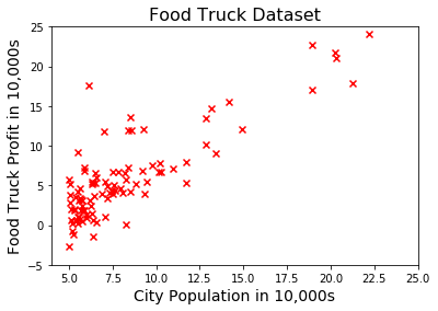
我们看Andrew Ng的机器学习课程的一个回归问题(regression problem),此问题的目标是训练一个模型以便准确预测一个城市中的餐车的利润。
我们的数据集中的第一列是各个城市的人口,第2列则是该城市的餐车利润,比如下面是数据集中的前面的一些样本(数量都以10000为单位)
6.1101,17.592
5.5277,9.1302
8.5186,13.662
7.0032,11.854
5.8598,6.8233
...
我们要用数据集作为样本去构建我们的模型,可以先读取数据集
import numpy as np
import matplotlib.pyplot as plt

data = np.loadtxt('food_truck_data.txt', delimiter=",")
x = data[:, 0] # city populations
y = data[:, 1] # food truck profits
x,y都是一维向量,分别表示特征(feature )和目标变量( target variable)
fig, ax = plt.subplots()
ax.scatter(x, y, marker="x", c="red")
plt.title("Food Truck Dataset", fontsize=16)
plt.xlabel("City Population in 10,000s", fontsize=14)
plt.ylabel("Food Truck Profit in 10,000s", fontsize=14)
plt.axis([4, 25, -5, 25])
plt.show()
假设函数 Hypothesis Function
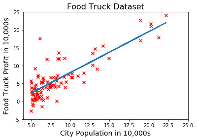
我们可以用一个直线(线性函数)来表示城市人口和利润之间的关系。即用下面的假设函数
\[h_\theta(x) = \theta_0+\theta_1x_1+\theta_2x_2+ ...+\theta_nx_n = (\theta_0,\theta_1,...\theta_n)(x_0,x_1,x_2,...x_n)^T \theta^Tx\]对于现在的问题,数据的特征只有1个,因此,可以写成下面的形式
\[h_\theta(x) = \theta_0+\theta_1x_1\]这个直线函数如图所示

假设函数可以看成x和未知参数(\(\theta\))的点积,未知参数(theta)可以表示成一个向量 \(\theta^T =(\theta_0,\theta_1,...\theta_n)\)
theta = np.zeros(2)
X = np.ones(shape=(len(x), 2))
X[:, 1] = x
predictions = X @ theta
print(predictions)
    [ 0.  0.  0.  0.  0.  0.  0.  0.  0.  0.  0.  0.  0.  0.  0.  0.  0.  0.
      0.  0.  0.  0.  0.  0.  0.  0.  0.  0.  0.  0.  0.  0.  0.  0.  0.  0.
      0.  0.  0.  0.  0.  0.  0.  0.  0.  0.  0.  0.  0.  0.  0.  0.  0.  0.
      0.  0.  0.  0.  0.  0.  0.  0.  0.  0.  0.  0.  0.  0.  0.  0.  0.  0.
      0.  0.  0.  0.  0.  0.  0.  0.  0.  0.  0.  0.  0.  0.  0.  0.  0.  0.
      0.  0.  0.  0.  0.  0.  0.]
训练模型就是最小化一个Cost Function(代价函数),这个代价就是就是测量目标值\(y\)和用训练模型得到的预测值之间\(h_\theta(x)\)的误差。
代价函数Cost Function可以表示成下面的形式
\[J(\theta) = \frac{1}{2m}\sum_{n=1}^{m}(h_\theta(x^{(i)})-y^{(i)})^2\]其中m表示样本的个数。
计算Cost Function的Python代码如下
def cost(theta, X, y):
    predictions = X @ theta
    squared_errors = np.square(predictions - y)
    return np.sum(squared_errors) / (2 * len(y))

print('The initial cost is:', cost(theta, X, y))
The initial cost is: 32.0727338775
梯度下降算法Gradient Descent Algorithm
为了求解未知的模型参数\(\theta\),可以用梯度下降法来迭代地求解:
\[\theta_j: = \theta_j -\alpha\frac{1}{m}\sum_{n=1}^{m}(h_\theta(x^{(i)})-y^{(i)})x_j^{(i)}\]def gradient_descent(X, y, alpha, num_iters):
num_features = X.shape[1]
theta = np.zeros(num_features) # initialize model parameters
for n in range(num_iters):
predictions = X @ theta # compute predictions based on the current hypothesis
errors = predictions - y
gradient = X.transpose() @ errors
theta -= alpha * gradient / len(y) # update model parameters
return theta # return optimized parameters
我们用这个函数训练我们的模型并画出假设函数
theta = gradient_descent(X, y, 0.02, 600)   # run GD for 600 iterations with learning rate = 0.02
predictions = X @ theta                     # predictions made by the optimized model
ax.plot(X[:, 1], predictions, linewidth=2)  # plot the hypothesis on top of the training data
fig
调试Debugging
对于只有1个特征的数据,我们可以画出拟合的曲线,通过视觉直接观察拟合的模型是否准确。但是对于1个特征的数据,则不可能轻松可视化拟合的模型。怎么才能知道结果如何呢?
一个简单的方法是绘制cost代价函数曲线,看看拟合模型的预测结果的cost值是否在不断下降?具体步骤是
1.  修改梯度下降法在每次迭代结束后记录cost值(Modify the gradient descent function to make it record the cost at the end of each iteration.)
2. 当梯度下降法完成后绘制“代价历史(cost history)”(Plot the cost history after the gradient descent has finished.)
3. 躺在你的座位上看看"代价cost"是否随着时间在下降(Pat yourself on the back if you see that the cost has monotonically decreased over time.)
修改的梯度下降算法
def gradient_descent(X, y, alpha, num_iters):
    cost_history = np.zeros(num_iters)          # create a vector to store the cost history
    num_features = X.shape[1]
    theta = np.zeros(num_features)
    for n in range(num_iters):
        predictions = X @ theta
        errors = predictions - y
        gradient = X.transpose() @ errors
        theta -= alpha * gradient / len(y)
        cost_history[n] = cost(theta, X, y)     # compute and record the cost
    return theta, cost_history                  # return optimized parameters and cost history
我们试试不同的学习率(learning rates)0.01 , 0.015, 0.02。对每个学习率绘制其对应的“代价历史(cost history)”
plt.figure()
num_iters = 1200
learning_rates = [0.01, 0.015, 0.02]
for lr in learning_rates:
    _, cost_history = gradient_descent(X, y, lr, num_iters)
    plt.plot(cost_history, linewidth=2)
plt.title("Gradient descent with different learning rates", fontsize=16)
plt.xlabel("number of iterations", fontsize=14)
plt.ylabel("cost", fontsize=14)
plt.legend(list(map(str, learning_rates)))
plt.axis([0, num_iters, 4, 6])
plt.grid()
plt.show()
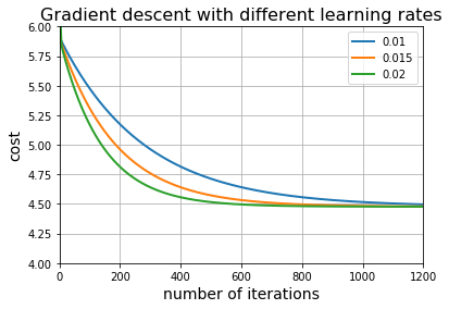
对这几个学习率,梯度下降都能能正确地工作,并且发现学习率低的需要更多的迭代次数。
那么能不能用更大的学习率呢
learning_rate = 0.025
num_iters = 50
_, cost_history = gradient_descent(X, y, learning_rate, num_iters)
plt.plot(cost_history, linewidth=2)
plt.title("Gradient descent with learning rate = " + str(learning_rate), fontsize=16)
plt.xlabel("number of iterations", fontsize=14)
plt.ylabel("cost", fontsize=14)
plt.axis([0, num_iters, 0, 6000])
plt.grid()
plt.show()
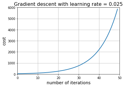
结果不妙!说明学习率太大了,尽管梯度下降法总能沿着正确的方向前进,但由于学习率太大,前进的步伐太大,越过了目标值(最佳解),因此代价发散而不是收敛。
目前学习率0.02比较合适,它能以较少的迭代次数收敛(最小化目标函数值)
Prediction预测
现在我们可以用拟合的模型(参数)去预测某个特定城市的餐车利润了。比如
theta, _ = gradient_descent(X, y, 0.02, 600)    # train the model训练模型
test_example = np.array([1, 7])                 # pick a city with 70,000 population as a test example
                                                # 选择7万人的城市作为一个测试例子
prediction = test_example @ theta               # use the trained model to make a prediction  预测结果
print('For population = 70,000, we predict a profit of $', prediction * 10000);
For population = 70,000, we predict a profit of $ 45905.6621788
 支付宝打赏
支付宝打赏
 微信打赏
微信打赏
您的打赏是对我最大的鼓励!