注:我没有完全照着原文翻译,省略了一些字句,使得尽量内容简洁。
学习曲线(Learning Curves) 分析机器学习模型的Bias-Variance方面很有用。本文用一个简单的线性回国模型作为案例说明如何用学习曲线提高改进模型。
学习曲线介绍 Introduction to Learning Curves
学习曲线用于在训练模型的时候显示随着训练样本的增加训练和验证模型误差的变化情况
-
If a model is balanced, both errors converge to small values as the training sample size increases.
-
If a model has high bias, it ends up underfitting the data. As a result, both errors fail to decrease no matter how many examples there are in the training set.
-
If a model has high variance, it ends up overfitting the training data. In that case, increasing the training sample size decreases the training error but it fails to decrease the validation error.
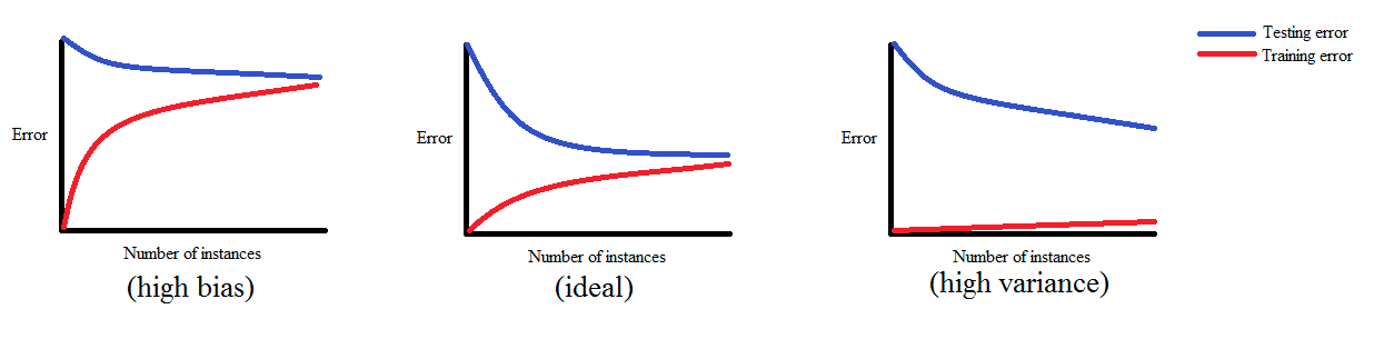
可以参考这个图理解Bias-Variance

Problem Definition and Dataset
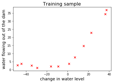
这是 Andrew Ng机器学习课程的另外一个例子,给定reservoir的水级别(level),预测流出Dam的水流量。因为原始数据集是一个MAtlab作业,所以数据集是MAtlab文件格式,我们可以用 SciPy.的loadman来读取这个文件,当然也要包含 NumPy 和 Matplotlib来进行矩阵运算和可视化.
import numpy as np
import matplotlib.pyplot as plt
import scipy.optimize as opt # we'll need this later
import scipy.io as sio

dataset = sio.loadmat("water.mat")
x_train = dataset["X"]
x_val = dataset["Xval"]
x_test = dataset["Xtest"]

# squeeze the target variables into one dimensional arrays
y_train = dataset["y"].squeeze()
y_val = dataset["yval"].squeeze()
y_test = dataset["ytest"].squeeze()
数据集包含3种样本:
-
The training sample consists of x_train and y_train.
-
The validation sample consists of x_val and y_val.*
-
The test sample consists of x_test and y_test.
注意:我们需要显式地将目标变量 (y_train, y_val and y_test) 转化为一维向量,因为原始的是mat矩阵。
让我们画一些训练样本看看
fig, ax = plt.subplots()
ax.scatter(x_train, y_train, marker="x", s=40, c='red')
plt.xlabel("change in water level", fontsize=14)
plt.ylabel("water flowing out of the dam", fontsize=14)
plt.title("Training sample", fontsize=16)
plt.show()
游戏计划The Game Plan
很明显,x,y之间存在的是一种非线性关系,但我们先训练一个线性模型以便看看高bias的模型学习曲线是什么样的?
然后我们训练一个比线性模型更灵活的多项式回归模型(polynomial regression model),看看具有高Variance的学习曲线
最后我们在多项式回归模型加入一个 规范项(regularization), 看看平衡的模型的学习曲线又是什么样的?
Linear Regression
上一篇我们用梯度下降法训练一个线性回归模型,但这一次,我们用scipy.optimize的优化函数fmin_cg来求解模型参数,这个算法比梯度下降法快且不需要我们试验学习率参数(select a learning rate by trial and error.)
fmin_cg需要2个函数参数:一个函数计算假设的代价cost,另一个函数计算这个cost函数关于未知参数的梯度。我们可以利用前一篇博文的代码
-
Cost函数可以直接拿过来
-
从gradient_descen函数中可以抽取一部分代码来计算梯度
def cost(theta, X, y):
    predictions = X @ theta
    return np.sum(np.square(predictions - y)) / (2 * len(y))

def cost_gradient(theta, X, y):
    predictions = X @ theta
    return X.transpose() @ (predictions - y) / len(y)

def train_linear_regression(X, y):
    theta = np.zeros(X.shape[1]) # initialize model parameters with zeros
    return opt.fmin_cg(cost, theta, cost_gradient, (X, y), disp=False)
我们看到在计算cost时,需要样本矩阵\(X\)和模型参数\(\theta\)进行矩阵相乘,因此,它们的维度应该匹配,和上一篇博文一样,我们需要对样本矩阵(比如x_train)插入值为1的一列。可以写一个小的实用函数来做这件事
def insert_ones(x):
    X = np.ones(shape=(x.shape[0], x.shape[1] + 1))
    X[:, 1:] = x
    return X
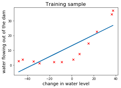
现在我们开始训练这个线性回归模型并在样本上画出拟合的直线
X_train = insert_ones(x_train)
theta = train_linear_regression(X_train, y_train)
hypothesis = X_train @ theta
ax.plot(X_train[:, 1], hypothesis, linewidth=2)
fig
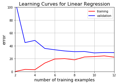
线性回归的学习曲线 Learning Curves for Linear Regression
为了得到学习曲线,我们从2个样本开始训练,每次增加1个样本进行训练。用每次训练得到的模型计算训练误差和验证误差。
def learning_curves(X_train, y_train, X_val, y_val):
    train_err = np.zeros(len(y_train))
    val_err = np.zeros(len(y_train))
    for i in range(1, len(y_train)):
        theta = train_linear_regression(X_train[0:i + 1, :], y_train[0:i + 1])
        train_err[i] = cost(theta, X_train[0:i + 1, :], y_train[0:i + 1])
        val_err[i] = cost(theta, X_val, y_val)
    plt.plot(range(2, len(y_train) + 1), train_err[1:], c="r", linewidth=2)
    plt.plot(range(2, len(y_train) + 1), val_err[1:], c="b", linewidth=2)
    plt.xlabel("number of training examples", fontsize=14)
    plt.ylabel("error", fontsize=14)
    plt.legend(["training", "validation"], loc="best")
    plt.axis([2, len(y_train), 0, 100])
    plt.grid()
为了使用这个函数,和x_train一样,我们需要修改x_val的大小(即插入值为1的一列)。然后调用这个learning_curves来得到并绘制学习曲线
X_val = insert_ones(x_val)
plt.title("Learning Curves for Linear Regression", fontsize=16)
learning_curves(X_train, y_train, X_val, y_val)
Polynomial Regression
现在我们讨论多项式回归
Feature Mapping
为了训练一个多项式回归模型,我们需要将存在的特征人工地映射为多项式特征(注:即用原始特征的多项式项作为新的特征)。
因为我们的样本只有一个特征x1,即水的级别level,我们可以通过对这个x1特征的指数次方得到它的多项式特征。即\(x_1^i\)
def poly_features(x, degree):
    X_poly = np.zeros(shape=(len(x), degree))
    for i in range(0, degree):
        X_poly[:, i] = x.squeeze() ** (i + 1);
    return X_poly
现在我们对training, validation and test 的样本生成8次方的多项式特征构造新的特征矩阵
x_train_poly = poly_features(x_train, 8)
x_val_poly = poly_features(x_val, 8)
x_test_poly = poly_features(x_test, 8)
特征规范化Feature Normalization
当我们观察我们生成的多项式特征矩阵时,我们发现还有一些小问题。
print(x_train_poly[:4, :])
[[ -1.59367581e+01   2.53980260e+02  -4.04762197e+03   6.45059724e+04
   -1.02801608e+06   1.63832436e+07  -2.61095791e+08   4.16102047e+09]
 [ -2.91529792e+01   8.49896197e+02  -2.47770062e+04   7.22323546e+05
   -2.10578833e+07   6.13900035e+08  -1.78970150e+10   5.21751305e+11]
 [  3.61895486e+01   1.30968343e+03   4.73968522e+04   1.71527069e+06
    6.20748719e+07   2.24646160e+09   8.12984311e+10   2.94215353e+12]
 [  3.74921873e+01   1.40566411e+03   5.27014222e+04   1.97589159e+06
    7.40804977e+07   2.77743990e+09   1.04132297e+11   3.90414759e+12]]
随着次数增加,其对应的多项式特征值会变得很大,,即使同一个指数的特性(同一列),其数值也是成数量级地变化。用这样的特征值不平衡的数据集去训练,cost代价函数会收敛得很慢。
在训练模型前,我们需要使得这些特征在尺度上应该尽可能相近。饮醋,我们需要做2步
- 每一列特征减去这一列的平均值
- 将每一列的值除以它们的平均方差,以便这些值位于[0,1]之间
特别需要注意的是: 我们必须用Train训练集中的平均值和方差对验证集和测试集做同样的处理,而不是单独进行规范化
train_means = x_train_poly.mean(axis=0)
train_stdevs = np.std(x_train_poly, axis=0, ddof=1)

x_train_poly = (x_train_poly - train_means) / train_stdevs
x_val_poly = (x_val_poly - train_means) / train_stdevs
x_test_poly = (x_test_poly - train_means) / train_stdevs

X_train_poly = insert_ones(x_train_poly)
X_val_poly = insert_ones(x_val_poly)
X_test_poly = insert_ones(x_test_poly)
最后,我们用train_linear_regression训练我们的多项式回归模型,然后绘制拟合的多项式曲线。因为多项式特征是作为独立的特征,训练一个多项式模型和训练一个多变量的线性回归模型是没有任何区别的。
def plot_fit(min_x, max_x, means, stdevs, theta, degree):
    x = np.linspace(min_x - 5, max_x + 5, 1000)
    x_poly = poly_features(x, degree)
    x_poly = (x_poly - means) / stdevs
    x_poly = insert_ones(x_poly)
    plt.plot(x, x_poly @ theta, linewidth=2)
    plt.show()

theta = train_linear_regression(X_train_poly, y_train)
plt.scatter(x_train, y_train, marker="x", s=40, c='red')
plt.xlabel("change in water level", fontsize=14)
plt.ylabel("water flowing out of the dam", fontsize=14)
plt.title("Polynomial Fit", fontsize=16)
plot_fit(min(x_train), max(x_train), train_means, train_stdevs, theta, 8)
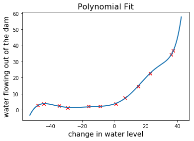
看起来是不是很准确?让我们再看看学习曲线
plt.title("Learning Curves for Polynomial Regression", fontsize=16)
learning_curves(X_train_poly, y_train, X_val_poly, y_val)
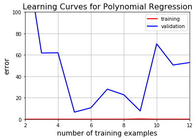
现在看到这是过拟合overfitting,即使训练误差很低,验证误差根本不收敛。
因此,我们在灵活性的同时需要某种东西,显然,线性回归不可能更多的灵活性,我们需要通过”正则化regularization “降低多项式回归的灵活性。
Regularized Polynomial Regression正则化多项式回归
Regularization允许我们在训练时通过对过大的\(\theta\)更大的惩罚避免过拟合。
添加了Regularization的目标函数是
\[J(\theta) = \frac{1}{2m}\sum_{i=1}^{m}(h_\theta(x^{(i)})-y^{(i)})^2 + \frac{\lambda}{2m}\sum_{j=1}^{n}(\theta_j^2)\]其梯度为:
\(\frac{J(\theta)}{\theta_0} = \frac{1}{m}\sum_{i=1}^{m}(h_\theta(x^{(i)})-y^{(i)})x_j^{(i)}\) for \(j=0\)
\(\frac{J(\theta)}{\theta_j} = \frac{1}{m}\sum_{i=1}^{m}(h_\theta(x^{(i)})-y^{(i)})x_j^{(i)} +\frac{\lambda}{m}\theta_j\) for \(j!=0\)
注意,我们没有惩罚\(\theta_0\),因为它和模型的灵活性无关
当然,我们通过一个正则化参数$$\lambda$将这些变化反映到python实现中.
def cost(theta, X, y, lamb=0):
    predictions = X @ theta
    squared_errors = np.sum(np.square(predictions - y))
    regularization = np.sum(lamb * np.square(theta[1:]))
    return (squared_errors + regularization) / (2 * len(y))

def cost_gradient(theta, X, y, lamb=0):
    predictions = X @ theta
    gradient = X.transpose() @ (predictions - y)
    regularization = lamb * theta
    regularization[0] = 0 # don't penalize the intercept term
    return (gradient + regularization) / len(y)
train_linear_regression 和 learning_curves也要做相应的修改
def train_linear_regression(X, y, lamb=0):
    theta = np.zeros(X.shape[1])
    return opt.fmin_cg(cost, theta, cost_gradient, (X, y, lamb), disp=False)

def learning_curves(X_train, y_train, X_val, y_val, lamb=0):
    train_err = np.zeros(len(y_train))
    val_err = np.zeros(len(y_train))
    for i in range(1, len(y_train)):
        theta = train_linear_regression(X_train[0:i + 1, :], y_train[0:i + 1], lamb)
        train_err[i] = cost(theta, X_train[0:i + 1, :], y_train[0:i + 1])
        val_err[i] = cost(theta, X_val, y_val)
    plt.plot(range(2, len(y_train) + 1), train_err[1:], c="r", linewidth=2)
    plt.plot(range(2, len(y_train) + 1), val_err[1:], c="b", linewidth=2)
    plt.xlabel("number of training examples", fontsize=14)
    plt.ylabel("error", fontsize=14)
    plt.legend(["Training", "Validation"], loc="best")
    plt.axis([2, len(y_train), 0, 100])
    plt.grid()
现在我们可以训练正则化的多项式回归模型(regularized polynomial regression model.)了.设置\(\lambda=1\)并在训练样本上绘制拟合的多项式曲线
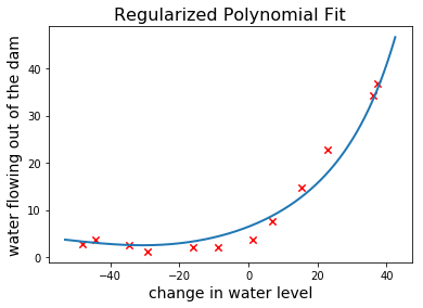
很清楚,假设函数比没有正则项的少了一些灵活性。让我们绘制学习曲线,观察bias-variance的平衡程度
plt.title("Learning Curves for Regularized Polynomial Regression", fontsize=16)
learning_curves(X_train_poly, y_train, X_val_poly, y_val, 1)
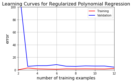 明显的,这是我们目前提出的最好的模型
Choosing the Optimal Regularization Parameter
上面通过设置\(\lambda=1\)改进了模型,我们还可以通过优化\(\lambda\)的值得到更好的模型,即通过对一组不同的\(\lambda\)进行训练,然后找出使得验证误差最小的那个\(\lambda\)
lambda_values = [0, 0.001, 0.003, 0.01, 0.03, 0.1, 0.3, 1, 3, 10];
val_err = []
for lamb in lambda_values:
    theta = train_linear_regression(X_train_poly, y_train, lamb)
    val_err.append(cost(theta, X_val_poly, y_val))
plt.plot(lambda_values, val_err, c="b", linewidth=2)
plt.axis([0, len(lambda_values), 0, val_err[-1] + 1])
plt.grid()
plt.xlabel("lambda", fontsize=14)
plt.ylabel("error", fontsize=14)
plt.title("Validation Curve", fontsize=16)
plt.show()
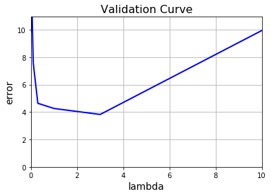
我们看到,最佳值是\(\lambda=3\)
评估测试误差Evaluating Test Errors
评估优化模型的一个好的实践是用不同于训练集和验证集之外的测试集去检查。让我们再一次训练模型并计算其在测试集上的误差
X_test = insert_ones(x_test)
theta = train_linear_regression(X_train, y_train)
test_error = cost(theta, X_test, y_test)
print("Test Error =", test_error, "| Linear Regression")

theta = train_linear_regression(X_train_poly, y_train)
test_error = cost(theta, X_test_poly, y_test)
print("Test Error =", test_error, "| Polynomial Regression")

theta = train_linear_regression(X_train_poly, y_train, 3)
test_error = cost(theta, X_test_poly, y_test)
print("Test Error =", test_error, "| Regularized Polynomial Regression (at lambda = 3)")
Test Error = 32.5057492449 | Linear Regression
Test Error = 16.9349317906 | Polynomial Regression
Test Error = 3.85988781599 | Regularized Polynomial Regression (at lambda = 3)
 支付宝打赏
支付宝打赏
 微信打赏
微信打赏
您的打赏是对我最大的鼓励!