Dynamic Programming
Policy Evaluation (Prediction)
For a given policy \(\pi\) compute the state–value function \(V^{\pi}\)
\[\begin{equation}\begin{split} V^{\pi}(s) = E_{\pi}[r_{t+1}+ \gamma V^{\pi}(s_{t+1}) \vert s_t=s]\\ =\sum_{a\in A} \pi (a\vert s)(R(s,a)+\gamma \sum_{s' \in S}P(s' \vert s,a) V^{\pi}(s')) \end{split}\end{equation}\]A system of jSj simultaneous linear equations Solution in matrix notation (complexity \(O(n^3))\):
\[V^{\pi} = (1- \gamma P^{\pi})^{-1} R^{\pi}\]Iterative Policy Evaluation
Iterative application of Bellman expectation backup
\[V_0\rightarrow V_1\rightarrow V_2\rightarrow ...\rightarrow V_k\rightarrow ...\rightarrow V^{pi}\]A full policy–evaluation backup:
\[V_{k+1}(s) =\sum_{a\in A} \pi (a\vert s)(R(s,a)+\gamma \sum_{s' \in S}P(s' \vert s,a) V_{k}(s'))\]A sweep consists of applying a backup operation to each state Using synchronous backups
- At each iteration k + 1
- For all states \(s\in S\)
- Update \(V^{k+1}(s)\) from \(V^{k}(s^{\prime})\)

Policy Improvement
Policy Improvement Theorem
For some state s we would like to know whether or not we should change the policy to deterministically choose an action \(a \neq \pi(s)\),We know how good it is to follow the current policy from s—that is \(v_{\pi}(s)\)—but would it be better or worse to change to the new policy ? One way to answer this question is to consider selecting a in s and thereafter following the existing policy, \(\pi\)
\[\begin{equation}\begin{split} Q_{\pi}(s,a) = E[r_{t+1}+ \gamma V^{\pi}(s_{t+1}) \vert s_t=s, a]\\ = \sum_{s^{\prime},r} p (s^{\prime},r\vert s,a) [r+\gamma v_{\pi}(s^{\prime}) ] \end{split}\end{equation}\]Let \(\pi\) and \(\pi^{\prime}\) be any pair of deterministic policies such that
\[Q^{\pi}(s,\pi^{\prime}(s)) \geq V^\pi(s), \forall s\in S\]Then the policy \(\pi^{\prime}\) must be as good as, or better than \(\pi\)
\[V^{\pi^{\prime}} (s)) \geq V^\pi(s)\]Proof.
\[\begin{equation}\begin{split} V^{\pi}(s) \leq Q^{\pi}(s,\pi^{\prime}(s) ) = E_{\pi^{\prime}}[r_{t+1}+ \gamma V^{\pi}(s_{t+1}) \vert s_t=s]\\ \leq E_{\pi^{\prime}}[r_{t+1}+ \gamma Q^{\pi}(s_{t+1},\pi^{\prime}(s_{t+1} ) \vert s_t=s]\\ \leq E_{\pi^{\prime}}[r_{t+1}+ \gamma r_{t+2}+\gamma^2 Q^{\pi}( s_{t+2},\pi^{\prime}(s_{t+2} ) \vert s_t=s]\\ \leq E_{\pi^{\prime}}[r_{t+1}+ \gamma r_{t+2}+ \gamma^2 r_{t+3}+\cdots \vert s_t=s] = V^{\pi^{\prime}}(s) \end{split}\end{equation}\]Policy Iteration
What if improvements stops ( \(V^{\pi^{\prime}} = V^{\pi} )\) ?
\[Q^{\pi}(s,\pi^{\prime}(s)) = \max_{a\in A} Q^{\pi}(s,a) = Q^{\pi}(s,\pi(s)) = V^{\pi}(s)\]But this is the Bellman optimality equation, Therefore
\[V^{\pi}(s) = V^{\pi^{\prime}}(s) = V^*(s)\]So \(\pi\) is an optimal policy!
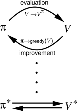
\[\pi_0 \rightarrow V^{\pi_0} \rightarrow \pi_1 \rightarrow V^{\pi_1}\rightarrow \cdots\rightarrow \pi^* \rightarrow V^* \rightarrow \pi^*\]

Value Iteration
One drawback to policy iteration is that each of its iterations involves policy evaluation, which may itself be a protracted iterative computation requiring multiple sweeps through the state set.
In fact, the policy evaluation step of policy iteration can be truncated in several ways without losing the convergence guarantees of policy iteration. One important special case is when policy evaluation is stopped after just one sweep (one update of each state). This algorithm is called value iteration. It can be written as a particularly simple update operation that combines the policy improvement and truncated policy evaluation steps:
\[\begin{equation}\begin{split} V_{k+1}(s) = \max _{a\in A } E_{\pi}[r_{t+1}+ \gamma V_{k}(s_{t+1}) \vert s_t=s]\\ = \max_{a\in A} \sum_{s^{\prime},r} p (s^{\prime},r\vert s,a) [r+\gamma v_{k}(s^{\prime}) ] \end{split}\end{equation}\]
您的打赏是对我最大的鼓励!
 支付宝打赏
支付宝打赏  微信打赏
微信打赏